Dataspace|COVID|Mod 1

COVID

Exploring Racial Disparities in New York City's Stop-and-Frisk Policies

By Shonda Kuiper. Contributors: Yusen He, Allie Jones, Shreyas Agrawal '24, Bowen Mince '22, Wagih Henawi '22, Adam Solar '22, Ying Long '17, Krit Petrachaianan '17, Zachary Segall '18

Key Question:

How can models help us make informed decisions about pandemic planning?

Part 1A: Introduction

Think back to the early days of the COVID-19 pandemic, shortly after a novel coronavirus disease was first identified and reported on December 31, 2019. Within weeks, the virus had spread to dozens of countries, with cases climbing quickly. Hospitals rapidly became overloaded and short-staffed, ICU beds were full, and healthcare workers were put under an immense mental and physical toll, having to work overtime under psychological distress.

Numerous government organizations have been turning to epidemiologists to:

1) Understand and predict how the pandemic will progress, and

2) Determine which actions to take to prevent the spread of the disease.

This site will discuss both of these core ideas. While the model shown below is a simplified model, it is very similar to the models used by many government organizations in the early days of the pandemic.

Part 1B: SIR Model

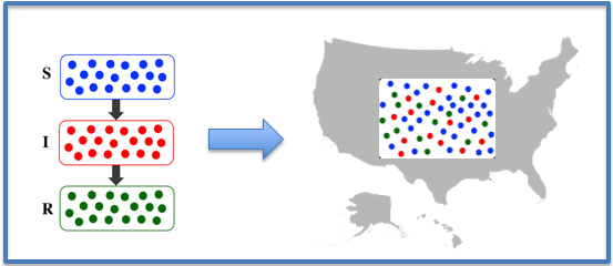
Epidemiologists often use SIR models to represent the spread of diseases. This is a compartment-based model, meaning each person in the population is considered to be within one of several compartments. In this model, each person in a population is considered to be either Susceptible (S), Infected (I), or Recovered/Removed (R). This means that at any given time, a person is either:

Susceptible to infection, meaning that they have not yet been infected.
Infected, meaning that they currently have the disease and are capable of spreading it to other susceptible people. In other words, they are contagious.
Recovered/Removed, meaning that the person is no longer contagious; they have either recovered from the disease or have died and been removed from the population. Either way, they are no longer infected or susceptible to infection.

Then, equations are used to determine how people in the population will move from susceptible to infected and from infected to recovered/removed.

Figure 1A: Compartmental SIR models are most common. At any given point in time, each person in the population can be located in exactly one compartment, although they can move between compartments over time.

Part 1C: Exploring the SIR Model

In any model, we start with multiple assumptions:

Population (N): We assume there are a fixed number of people in the population. In the case of COVID-19 modeling done for national governments, the population of interest is likely to be the total population of the country. However, SIR models can also be used to predict the spread of a disease in a smaller closed community, such as people on a cruise ship or in a prison.
Initial Infected (InfectedDay = 1): The number of people infected with the disease on the day that the model "starts".
Transmission Rate: A measure of how quickly the disease will spread. This is expressed as the number of susceptible people that each infected person will infect per day, on average. Transmission rate could be determined by factors such as:

The probability that a susceptible person who comes into contact with an infected person will themselves become infected.
The number of other people that a given person comes into contact with on any given day

Recovery Rate: A measure of how long people take to move from infected to recovered. This is expressed as the proportion of people who are currently infected who will move to the recovered/removed compartment per day.

Models also include implicit assumptions. A major assumption of the SIR model is that once a person has recovered from the disease, they cannot catch the disease again. Of course, we know now that recovering from COVID-19 does not provide a person with lifelong immunity to reinfection in the same way that recovering from, say, measles or chicken pox does, which makes it problematic to model COVID-19 with a basic SIR model such as this one. However, in early 2020 epidemiologists assumed that recovery from COVID-19 would confer such immunity.

Each one of the formally assumed values can dramatically influence the model. However, in reality, these values are not known, especially at the beginning of an epidemic. Thus, researchers must estimate each of the assumed values. Below is an app that illustrates a basic SIR model. Try changing the parameters to see how they affect the overall spread of the disease. Then, answer the questions to the right to check your understanding. By understanding this model and the calculations below, we can see why at the beginning of the pandemic the spread of COVID-19 was often represented as a "curve".

Calculation Details

Using the above app, set the initial conditions so that they fit the following assumed initial conditions. You can then verify the numbers found in the app with the calculations shown below.

Population: N = 5000
Initial Infected: InfectedDay = 1: 10
Transmission Rate: 1
Recovery Rate: 0.3

Calculating Recovered:

Recovered₂ = Recovered₁ + (Infected₁ * Recovery Rate)

3 = 0 + (10 * 0.3)

Calculating Infected:

Infected₂ = Infected₁ + (Infected₁ * Susceptible₁ * Transmission Rate)/N - Recovered₂

17 = 10 + (10 * 4990 * 1)/5000 - 3 (Rounded)

Calculating Susceptible:

Susceptible₂ = Susceptible₁ - (Infected₁ * Susceptible₁ * Transmission Rate)/N

4980 = 4990 - (10 * 4990 * 1)/5000 (Rounded)

Part 1D: How Public Policy Influence Model Assumptions

It’s one thing to study a graph, but you can really understand the nuance and complexity of the data when you manipulate it yourself! See if you can use the NYPD Bar Chart App to recreate Figure 1A and Figure 1B on your own. Then modify the graph to answer the questions below.

Let’s take a closer look at a couple of the parameters in our simple SIR model.

Transmission Rates

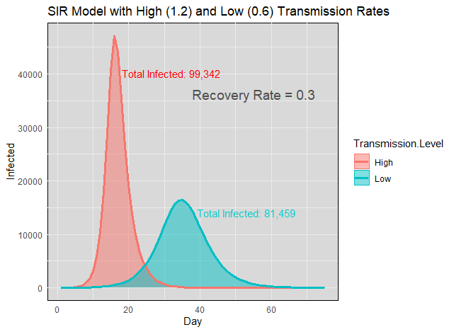
If you change the transmission rate in the graphing application above, you’ll notice that lowering the transmission rate by itself does not necessarily stop the spread of the disease. The true determinant of how many people will ultimately get the disease is the ratio between the transmission rate and the recovery rate. This is often referred to as the Reproducibility Number (R). This number tells us, on average, how many additional people one infected person will infect over the entire course of their infection. As you can see in the graph, if R is greater than 1—that is, if the transmission rate is greater than the recovery rate—then an epidemic will occur since more people are being infected than are recovering. If R is less than 1, then the disease will die out as more people are recovering then being infected. If R is very close to 1, there will be a constant rate of infections

The Reproducibility Number will change over the course of the epidemic; as people move from susceptible to recovered/removed, the number of susceptible people shrinks and each infected person will be able to cause fewer new infections. Thus epidemiologists often talk about R0, or the Reproducibility Number on day 0 when everyone in the population is still susceptible. You can also calculate Rt, or the Reproducibility Number on day t, or the Reproducibility Number on day t. As we can see in the graph, when the transmission rate is greater than recovery rate, we can see that Rt is initially greater than one and the number of people wh are infected every day increases. Then, after infections reach peak on day t and start to decrease, Rt is less than 1. One of the major challenges in SIR modeling is that the transmission rate is non-constant. It is time-dependent and can vary drastically.

Initial Infected

The initial infected parameter can also affect whether an outbreak will occur. Remember that for an epidemic to occur, each person who is infected must infect, on average, more than one additional person over the course of their infection. Let’s say the R0 for a particular disease is 1.33, and at present only one person is infected. That person can’t infect 1 and 1/3 of a person! Each whole person is either infected or not, so the calculations in the SIR model are rounded to the nearest whole number. With an R0 of 1.33, in an SIR model that person will only infect one other person (1.33 will round down to 1), who will also only infect one other person, and an epidemic will not occur. However, if 10 people are infected initially, they will infect a total of 13 people between them, who will infect a further 17 people, and the number of cases will grow into an epidemic. You can see this yourself using the graphing application or the calculations above.

Looking at the variability of SIR models

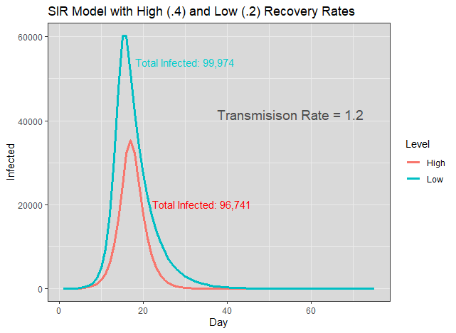
Predicting how the COVID-19 pandemic would progress quickly proved to be an incredibly challenging task. The images below represent possible scenarios that the CDC suggested early in the pandemic based on different possible values for R0, using SIR simulations with a population of 100,000. You can see from these images that altering the transmission rate and recovery rate even slightly caused drastic changes in the predicted outcome for the pandemic. “Flattening the curve” by reducing the transmission rate does reduce the total number of infections, but it still leads to a majority of the population being infected. The number of people infected on the peak day of infections is dramatically lower, reducing the strain on the healthcare system, but the trade-off is that the epidemic lasts longer.

It is important to note that changing the recovery rate has little effect on how long the epidemic will last or how many people will ultimately be infected, unlike changing the transmission rate.

Model Complexity and Assumptions

We must remember that the model we have been looking at is very basic. The differences between the possible predicted outcomes become even more apparent as researchers increase the complexity of the models by, for example, adding parameters to account for an incubation period for the disease, for quarantine or isolation measures, or for the possibility of reinfection. When there is great uncertainty around the correct numbers to use for the model inputs, or even around which parameters need to be included in the model, any predictions produced by these models will be very uncertain as well. This uncertainly prevents creating reliable projections for the course of the outbreak, which frustrates efforts to contain outbreaks and worsens the already devastating burdens on the healthcare system and the economy. Careful attention must be given to the assumptions made when using any model, whether it be an SIR or a statistical model.

Additional Resources

To view a more complex shiny app with more variables for modeling Covid, click here. Grinnell College students Senay Gockcebel, Britney He, Bowen Mince, and Linh Tang did a simulation study on a more complex model. See the paper here. The Github for it can be reached here.

Explore Other Stories

Data Stories

NYPD
Covid-19
Recidivism
Brexit

Stats Games

Racer
Greenhouse
Statistically Grounded
Psychic

Questions?

If you have any questions or comments, please email us at DASIL@grinnell.edu

This page was last updated on November 11th 2024.